mr_e_man wrote:[...]
It's interesting (but perhaps expected?) that the polynomials bulge outward rather smoothly, with smaller coefficients at the ends, and smallest at the highest-degree term.
[...]
This isn't always the case, but generally yes, that's expected. It's a similar phenomenon to
binomial expansions.
mr_e_man wrote:Do you know of accurate numerical algorithms for solving multi-variable systems directly, without reducing them to single-variable equations and exploding the polynomial sizes? I can see a few possible ways to generalize Newton's method.
Actually, reduction to univariate polynomials is just a matter of presentation. Note that multi-variable
linear systems are "trivial" to solve with Gaussian elimination, for which there are plenty of implementations out there. The trouble with many polyhedral / polytopal constructions is that they involve non-linear systems. Mostly quadratic systems, but mathematically speaking, quadratic systems are equivalent to polynomial systems of arbitrary degree (because you can always introduce a new variable y and add the equation y = x^2, so quadratic systems can encode polynomial equations of arbitrary degree).
Polynomial systems are in general very difficult to solve, even when the starting equations appear to be "simple quadratics" (which is the case with most polytopal constructions). Unlike linear systems, where the complexity of the solution generally is proportional to the complexity of the input system, polynomial systems can have solutions that are exponential (or worse) in complexity relative to the input system.
Generally, solution proceeds by first computing a so-called Gröbner basis, which is the polynomial equivalent of row-echelon form for linear systems, then extracting solutions from there using various known transformations. Here, "solution" can mean different things; usually it means a presentation from which it is relatively simple to compute numerical approximations to any desired accuracy. I chose univariate polynomials because in simple cases, it's the most concise way of presenting the solution that allows extraction of numerical values to arbitrary precision. But as you can see, sometimes the univariate representation is not very useful, in that the size of the solution is impractically large relative to the size of a numerical approximation! Generally, coefficient sizes can be exponential in the complexity of the input. It's not the only representation, however. There's something called a rational univariate representation, in which you introduce an extra variable that has a polynomial relationship with the input variables, and express the solution in terms of this variable. Generally, the coefficient sizes are linear in the complexity of the solution, rather than exponential. I've yet to find an easy implementation of this, however, because choosing the right variable to introduce is not a trivial task, and not easily automated; and the size of the solution does depend very much on the choice of this variable.
There is also the approach of purely numerical solutions, where you start by inputting a set of guessed solution values, which is then iteratively refined using the defining equations. This approach has drawbacks, however. Polynomial systems generally are not "well-behaved" like linear systems; polynomials can have multiple solutions, and if you start with the wrong set of initial values, it may "miss" the solution, diverge, or if there are multiple solutions it may find any arbitrary one without any indication of the existence or number of other solutions. Polynomial systems also tend to be numerically unstable, meaning an iterative system may accumulate roundoff errors that either overwhelm the algorithm (in the extreme case, produces nonsensical values), or else converge too slowly to be of practical use. These problems apply not just to polynomial systems; even pure Newton's method on a function of a single variable may fail to converge, or hard to control where it converges in the case of multiple solutions, depending on what initial values you give it, and how the function behaves around the initial value.
One possible hybrid approach is to start with the Gröbner basis computation, but instead of outputting the solution polynomials as-is, use a polynomial root solver to extract numerical values to the desired precision and output that instead. That's what I've chosen with sphenohexonacingulum. This way, you let the computer deal with the crazy huge coefficients behind the scenes, and give you nice decimal approximations to any desired accuracy.
Of course, the Gröbner basis method / polynomial presentation presumes a reliable polynomial root-finding algorithm. Since polynomials generally have multiple roots, after the Gröbner basis is computed you still have the question of which polynomial root represents a solution. For this, you need a reliable algorithm for separating the roots and any potential multiplicities so that you can apply a numerical algorithm to reliable extract the numerical values (otherwise you run into the multiple root problem where something like Newton's method may fail to converge, or converge to the wrong root). Fortunately there are standard methods here that are widely used. One approach I know of is to compute a Sturm sequence to bracket the polynomial's roots, then use a numerical root-finder within each bracket to extract the value of the root.
For my purposes, I use Singular for the Gröbner basis computation (for 0-dimensional polynomial systems, it implements the super-fast FGLM algorithm, which first computes the Gröbner basis using an "easy" monomial ordering, then transforms it into lexicographic ordering as a second step -- computing Gröbner basis in lex ordering is generally very expensive, very slow, and often super-exponential in complexity). Then I use Maxima to compute polynomial roots -- it supports arbitrary-precision floats; although the default settings only give about 5-6 digits' accuracy, with correct configuration it can compute the roots to any number of digits. AFAIK Maxima uses Sturm sequences to bracket roots, then some kind of root-finder to compute the values, probably Newton's method or one of the hybrid methods like Brett's method. Funnily enough, Maxima internally works with rational approximations, but that's not a problem since with the right configuration it will automatically convert that to a decimal approximation up to the desired precision.
So yeah, polynomial systems are not easy to work with. Even a seemingly simple-looking system can explode in complexity, like we see here with sphenohexonacingulum.


I only glanced at the posts, didn't follow through in detail. But it does look like rigidity in all likelihood does apply to 4D and above. (But probably only in the convex case -- see below.)
Which means in 4D and above, you won't find the kind of arbitrary flexibility with degree ≥4 vertices that you find in 3D. So any CRF crown jewels in 4D would have to come from other directions, or be based on 3D crown jewels. Which also means that the set of possibilities of 4D CRF crown jewels is
discrete, and may be amenable to brute-force search. Though I'm skeptical about the feasibility of brute-force set without further refinement / restrictions; given the 300+ million CRFs generated by non-adjacent diminishings of the 600-cell alone, some restriction of scope will be necessary otherwise the algorithm may just get stuck enumerating 600-cell diminishings.

One approach, given the rigidity theorem, is to start with a 3D crown jewel and then try to disprove the possibility of closing up in a CRF way (except for the trivial prism). Failure to disprove it may reveal some new avenues of construction that might potentially lead to undiscovered 4D crown jewels.
Somebody in this forum brought up years ago that we can use the rigidity theorem to pre-compute the set of all vertex figures that can be made from the 3D CRFs. Once we exclude certain known infinite families, this set should be finite. Once we have this set, we can brute-force all CRFs simply by enumerating all possible combinations of vertex figures, or use it as a filter to prune parts of the search tree when a partially-constructed vertex sports a combination of cells that isn't a subset of any member of this set. We can also start with a vertex figure that contains a 3D crown jewel, and iteratively try to find adjacent vertex figures that might eventually close up the polytope.
On an interesting side note, the rigidity theorem I think only applies to
convex polytopes. In 3D, there are certain non-convex polyhedra that have rigid faces but the polyhedron itself can deform continuously. Although the first such example was self-intersecting, it's possible to construct a similar polyhedron in a non-self-intersecting way. Now imagine building a 4D polytope out of these polyhedra as cells.
That may lead to 4D continuously-deformable vertices that can produce crown-jewel-like constructions -- albeit this would no longer be CRF since (some of) the cells would be non-convex.


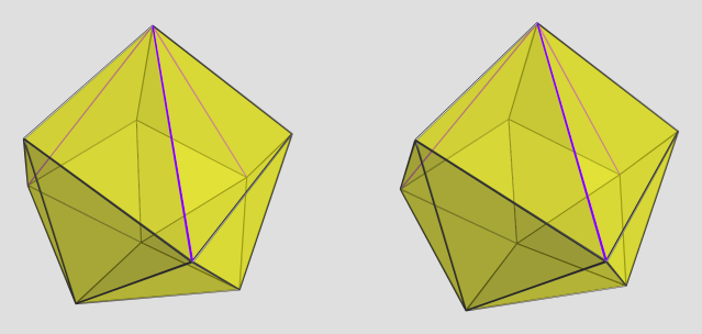


 (The little boy destroyed them before I could note them down, so I have to reconstruct them from memory!
  )
)
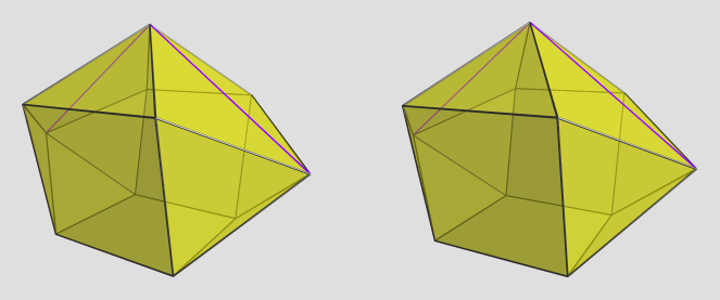
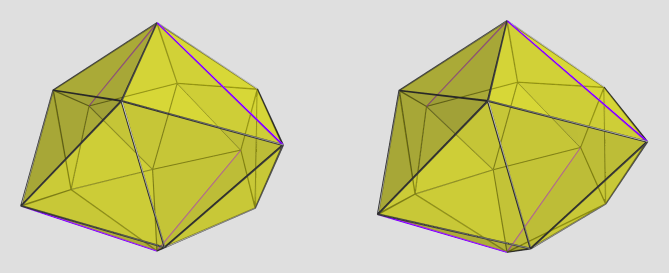
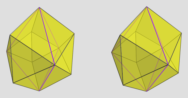


 The solver software I'm using, Singular, was able to handle these monsters just fine, albeit with some performance hits. Another helper CAD program, Maxima, was also able to extract roots from these beasts. However, the rest of my pipeline was defeated by the huge coefficients... I'd have to rework several key components to use BigInt's and BigFloat's in order to be able to get useful coordinates out of this beast.

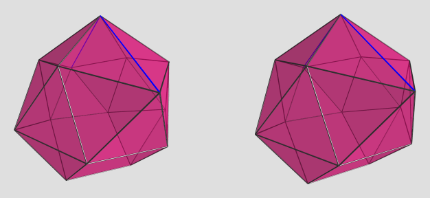

 Well, actually, technically it "only" takes ~15 mins to solve the system; the 3 hours is because the helper program I wrote does things the stupid way by recomputing the system once per unknown, so that's 15 mins multiplied by 13.